To freeze multiple rows (starting with row 1), select the row below the last row you want frozen and click Freeze Panes. To freeze multiple columns, select the column to the right of the last column you want frozen and click Freeze Panes. Say you want to freeze the top four rows and leftmost three columns.

How do I lock filters in Excel?

On the worksheet, select just the cells that you want to lock. Bring up the Format Cells popup window again (Ctrl+Shift+F). This time, on the Protection tab, check the Locked box and then click OK.

How do I freeze cells in Excel?

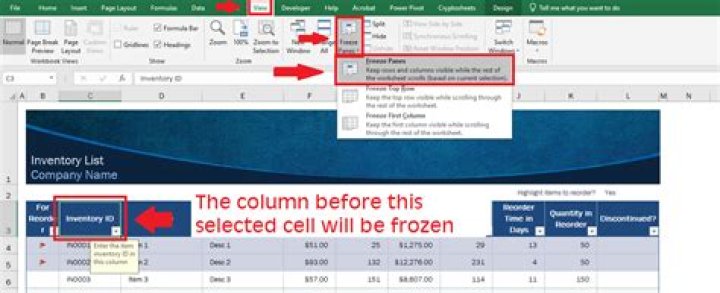
1. Select the cell below the rows and to the right of the columns you want to keep visible when you scroll.
2. Select View > Freeze Panes > Freeze Panes.

How do you lock cells so they don't move when sorting?

1. Select the row below the row(s) you want to freeze. In our example, we want to freeze rows 1 and 2, so we’ll select row 3. …
2. Click the View tab on the Ribbon.
3. Select the Freeze Panes command, then choose Freeze Panes from the drop-down menu. …
4. The rows will be frozen in place, as indicated by the gray line.

How do you lock rows when filtering?

1. format the data as a table.
2. in the Table Tools contextual > Designs tab > Table Style Options: Turn on “Header Row” and “Filter button.
3. teach them to click on the “Filter button” (#1)
4. pick the sort order they want to use (#2)

How do I sort excel and keep rows together?

Then in the Ribbon, go to Home > Sort & Filter > Sort Largest to Smallest. 2. In the Sort Warning window, select Expand the selection, and click Sort. Along with Column G, the rest of the columns will also be sorted, so all rows are kept together.

Can you lock rows in Excel?

Excel 2016 Select the row below the row(s) you want to freeze (select row 6, if you want to freeze rows 1 to 5). On the View tab, click Freeze Panes > Freeze Panes.

What is the shortcut key to freeze rows in Excel?

1. To freeze the top row: ALT + W + F + R. Note that the top row gets fixed.
2. To freeze the first column: ALT + W + F + C. Note that the left-most column gets fixed.

How do I sort in Excel without mixing data?

Select a cell or range of cells in the column which needs to be sorted. Click on the Data tab available in Menu Bar, and perform a quick sort by choosing any one of the options under the Sort & Filter group, depending upon whether you want to sort in ascending or descending order.

How do I freeze 3 columns in Excel?

To lock multiple columns, select the column to the right of the last column you want frozen, choose the View tab, and then click Freeze Panes.

Article first time published on

How do I freeze specific cells in Excel 2010?

1. Select the column to the right of the columns you want frozen. …
2. Click the View tab.
3. Click the Freeze Panes command. …
4. Select Freeze Panes. …
5. A black line appears to the right of the frozen area.

Why can't I freeze panes in Excel?

Causes of Excel Freeze Panes Not Working: The causes of this issue are when your Excel worksheet is in the page layout view, when Windows protection is turned on and also when the Excel sheet is protected by the earlier versions of Excel. Because of all this issues, Excel Freeze Panes Not Work properly.

How do you lock rows so they stay together during sort?

If you want to freeze more than just one row or one column, click the cell in the spreadsheet that’s just to the right of the last column you want to freeze and just below the last row you want to freeze. Then, click the View tab and Freeze Panes. Click Freeze Panes again within the Freeze Panes menu section.

How do I freeze both the top row and first column?

1. From the View tab, Windows Group, click the Freeze Panes drop down arrow.
2. Select either Freeze Top Row or Freeze First Column.
3. Excel inserts a thin line to show you where the frozen pane begins.

How do I freeze rows in Excel spreadsheet?

1. On your computer, open a spreadsheet in Google Sheets.
2. Select a row or column you want to freeze or unfreeze.
3. At the top, click View. Freeze.
4. Select how many rows or columns to freeze.

How do I freeze multiple rows in Excel 2020?

To freeze multiple rows (starting with row 1), select the row below the last row you want frozen and click Freeze Panes. To freeze multiple columns, select the column to the right of the last column you want frozen and click Freeze Panes. Say you want to freeze the top four rows and leftmost three columns.

How do I filter in Excel without affecting other columns?

You don’t – that is the idea behind filters – It shows the data that meets specific criteria in one or more columns, and hides the rest. If you want to filter 1 column without affecting other columns, copy that column to a new blank worksheet.

How do you automatically sort data in Excel?

1. Select the columns to sort.
2. In the ribbon, click Data > Sort.
3. In the Sort popup window, in the Sort by drop-down, choose the column on which you need to sort.
4. From the Order drop-down, select Custom List.
5. In the Custom Lists box, select the list that you want, and then click OK to sort the worksheet.

How do I sort a column in Excel but keep intact rows?

Using the sort Function Click on Data and eventually sort. This will make sure that the rows are intact but the columns have changed. After this, the sort warning dialog will pop up. You are supposed to keep the Expand the selection option and after that click on sort.

How do I sort columns without messing up rows?

1. Click into any cell in the COLUMN you want to sort by within your list. (DO NOT highlight that column as this will sort that column only and leave the rest of your data where it is.)
2. Click on the DATA tab.
3. Click on either the Sort Ascending or Sort Descending. button.

How do I filter multiple columns in Excel at the same time?

1. Click Enterprise > Super Filter, see screenshot:
2. In the popped out Super Filter dialog box: (1.) …
3. After finishing the criteria, please click Filter button, and the data has been filtered based on multiple column criteria simultaneously, see screenshot:

How does filter function work in Excel?

The FILTER function “filters” a range of data based on supplied criteria. The result is an array of matching values from the original range. In plain language, the FILTER function will extract matching records from a set of data by applying one or more logical tests.

What does Alt 9 do in Excel?

To do thisPressAdd borders.Alt+H, BDelete column.Alt+H, D, CGo to the Formula tab.Alt+MHide the selected rows.Ctrl+9

What does Alt 14 do?

Just about everyone knows that Alt+Ctrl+Del interrupts the operating system, but most people don’t know that Alt+F4 closes the current window. So if you had pressed Alt+F4 while playing a game, the game window would have closed. It turns out there are several other handy keystrokes like that built into Windows.

What is the shortcut key of filter in Excel?

To turn filtering on or off, ensure a cell in the range is selected and then press Ctrl + Shift + L. If your data range contains any blank columns or rows, select the entire range of cells first. If you have converted a list to a table, the Filter menus should automatically appear.

How do I freeze two columns in Excel 2021?

1. Select the column to the right of the column you want to freeze.
2. Select the View tab and Freeze Panes.
3. Select Freeze Panes.

How do I freeze first and second column in Excel?

Under view, browse to find freeze panes. Click on freeze panes to reveal the list of options, select the first option which is freeze panes. This option will freeze or rather lock the two columns in a way that they will always remain visible even after scrolling down.

Why the freeze first column option is used in Excel?

The Excel Freeze Panes tool allows you to lock your column and/or row headings so that, when you scroll down or over to view the rest of your sheet, the first column and/or top row remain on the screen. The following steps show you how to use freeze panes in Excel 2016, 2013, 2010, or 2007.

How do I freeze the top row and first column in Excel 2010?

1. From the View tab, Windows Group, click the Freeze Panes drop down arrow.
2. Select either Freeze Top Row or Freeze First Column.
3. Excel inserts a thin line to show you where the frozen pane begins.

Why won't Excel let me freeze top row and first column?

NOTE: Freezing panes only works when you are in Normal View. To freeze the first row and column, open your Excel spreadsheet. Select cell B2. Then select the VIEW tab from the toolbar at the top of the screen and click on the Freeze Panes button in the Window group.

How do I filter exclude rows in Excel?

Right-click a row or column member, select Filter, and then Filter. In the left-most field in the Filter dialog box, select the filter type: Keep: Include rows or columns that meet the filter criteria. Exclude: Exclude rows or columns that meet the filter criteria.